Simmechanics: Simulating floor interaction/collision

I'll demonstrate how to simulate a floor in Simmechanics, this floor will prevent free falling (6 DOF) objects from falling below a threshold level ("the floor level"), i.e. I will simulate a collision/interaction between the free falling object and the floor.

I'll assume you have a basic understanding of how Simmechanics works. If you don't, you might want to check this post.

The problem

If you have used Simmechanics before, then you know it's an excellent toolbox for simulation of multibody dynamics. You can easily work with robotic arms, which are always fixed to the ground. But what happens when you want to work with legged robots, that can't be fixed to the ground. Well, then you run in a problem, if you don't fix any part of the robot to the ground, then the robot will fall and fall by action of the gravity. Removing the gravity is not an option, because you want to design the controllers of your robot with gravity compensation, even worse your robot will float if you simulate a zero gravity environment.

Let's develop a minimal model to illustrate the problem: a 6 DOF ball.

Illustrating the problem

We'll start by drawing the floor. Implement the following block diagram in Simulink.

Block diagram to visualize the floor.

Modify the Floor block parameters to match the following image, and also on the Visualization tab change the Body geometry option to "Equivalent ellipsoid from mass properties".

Parameters to draw a 1 meter radius floor.

Next, start a simulation. Activate the the Isometric View and the "Enable Automatic Expanding Fit".

Animation showing the floor as a 1 m radius disk.

Now, we add the free falling ball. Add more blocks to the model to match the following diagram.

Added a free falling ball to the model.

Next, modify the parameters of the Above Ground block and the Ball block, to match the following images. On the Visualization tab of the ball block also select "Equivalent ellipsoid from mass properties" on the Body geometry option.

Above Ground parameters	Ball parameters

Now simulate the system and observe the problem.

Ball falling through the floor.

The Idea

Known the problem, we must now create a solution. Let's begin by analyzing how the floor behaves. Ideally the floor is a rigid body that exerts enough force over adjacent bodies to prevent them from falling through. Now, perfect rigid bodies doesn't exist in the real world, all bodies deform when stressed or compressed. This means our floor model must be elastic, this can be modeled as a spring.

Our floor model can't be modeled only as a spring, otherwise will end with a trampoline. When we fall to the ground, we don't jump back to the sky, instead our potential energy dissipates as heat or as permanent deformation. This means our floor model must also have a dissipation element.

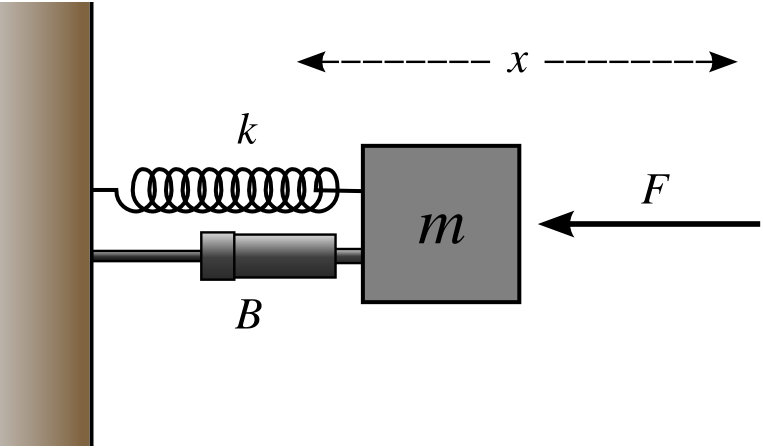
A mass-spring-damper system.

That description resembles a lot to a mass-spring-damper system. As you might know those system tend to vibrate, unless they are overdamped. This means our floor model must behave as an overdamped mass-spring-damper system. The final condition is that the free falling object must be the mass of the system, this means that our floor model doesn't really has a mass parameter. Other way to think of it is that the mass is detachable, and this mass is only affected by the spring and the damper when is at or below the floor level.

Implementing the floor interaction

First, let's enable some sensor/actuator ports on the free falling ball. These two ports must be located at the same point, at the bottom of the ball.

Adding sensor/actuator ports to the free falling ball.

The floor control diagram can be implemented as follows:

Floor Control Diagram.

The body sensor is configured to output the position in meters, while the body actuator is configured to exert force in newtons over the ball. Using a demuxer, we extract the Y component of the position, then we compare it to the floor level. If the Y position of the bottom of the ball is below the floor level, then we activate the spring-damper system represented by the gains 'k' and 'c', otherwise the floor exerts no force over the ball. The force developed by the spring damper system is exerted over the ball but only in the Y direction, thanks to a muxer and the body actuator.

The final step is selecting 'k' and 'c'. You need to considerate the following things:

• The damping ratio "c / 2 / sqrt(m * k)" should be greater than 1, to guarantee overdamping.
• The free falling body will sink a distance "m * g / k" into the ground, so you might want to increase 'k', right?
• But Increasing 'k', also increases the computation load of the simulation.

How do I select the parameters 'k' and 'c'? I first select 'k' balancing how much sinking and computation load can I tolerate. Then I compute 'c' using the biggest mass and choosing a damping ratio of 1.

The Results

I'll leave you with the simulation output.

Floor control enabled.

Ball interacting with the floor. (Y position)

As a closing remark, I must say that I have used this method in the simulation of a humanoid robot with positive results.

Simmechanics: Simulating multibody dynamics

In this post I'll cover how to simulate a multibody system (a "robotic arm") using the Simmechanics toolbox in Simulink, which is an extension of Matlab.

We'll build a simple "robotic arm" with 3 degree of freedom (DOF). Each DOF will be rotational and will be actuated by a "servomotor", which will be implemented as a closed loop PID position controller.

We won't build this one in this tutorial, as it requires too many steps. We'll build something simple to illustrate the method, then you can build this one on your own. 

I won't give you the final .mdl file, instead I'll give you all the necessary steps, so you can learn by doing.

OK, let's go hands on!

The environment

First, let's explore the environment. Launch Matlab and then open Simulink, either by using the command simulink in the command line or by clicking the simulink icon in the toolbar.

Launching Simulink

The Simulink Library Browser will open, here you'll find a bunch of building blocks that can be used to assemble Simulink models. We'll be using the first generation or legacy Simmechanics blocks located under the Simscape library. After you find these blocks, create a new model by clicking the blank page icon.

Starting a new simulink model

A new blank window, name untitled, will appear. This is the simulink model, we can drop blocks here to build models, which can later be simulated. You'll notice there is a play button which is disabled, that button starts the simulation.

A blank Simulink model...

Let's start by dropping a Ground block in the model, I'll explain what it does soon enough. You can find the Ground block inside the Bodies category of the Simmechanics blocks. Drag the Ground block and drop it inside the white are of the Simulink model.

Gaining ground on Simulink.

The coordinate system

Simulink uses an XYZ Cartesian coordinate system to describe the position of the bodies and Euler angles to describe the orientation of the bodies. Let's take a look at the global coordinate system (CS) by starting a simulation.

First, head to the menu > Simulation > Configuration Parameters. On the new window, go under the Simmechanics 1G (or simply Simmechanics) category and enable the animation by checking the "Show animation during simulation" checkbox.

Enabling animation.

Click the apply button and close the window. Now hit the play button (Start simulation). In the new window that pops out, select the isometric view as shown in the next image.

The Coordinate System and an empty animation.

You just did your first animation, there is nothing in it but the global coordinate system. Now, notice that the Y axis is pointing up, this is also the axis where the gravity acts (in the -Y direction). Some people, me included, tend to draw the Z axis pointing up and use the -Z direction for the gravity. Simulink doesn't follow this Z convention, so be careful.

The multibody paradigm: bodies and joints

As the name implies, multibody systems are composed of various bodies, where a body can be any rigid piece of matter. Two bodies are connected by joints, these joints allow one or more DOF (i.e. relative movement) between the bodies.

Most multibody system can be described as "open chains", i.e. as a series of bodies and joints that form a line or a tree, but not a loop. In Simmechanics, these chains must start with the Ground block, the Ground is a body with infinite mass and moment of inertia. Let's explore the Ground block by double-clicking it.

Ground block parameters

The Ground block is located at some [x, y, z] global position. This point is where other bodies will make a joint to the Ground. Leave the default [0, 0, 0] position.

The simplest example: A pendulum

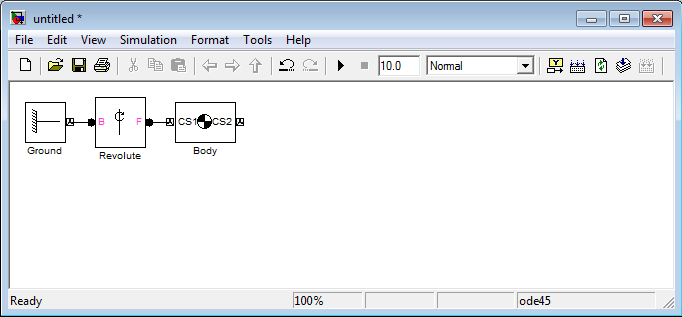
To better understand the joint and body system, let's start by building a simple pendulum system. Add a revolute block, located under the Joints category, and a body block, located under the Bodies category, to the Simulink model. Then, link these block by click dragging a line from one block to another, the final diagram should look like the following image.

Pendulum diagram.

Let's add parameters to the Body block. The Body will be a 1 meter zero-thickness bar with a mass of 1 Kg. Double click the Body block and modify the parameters to match the following image.

Bar parameters.

Click apply and close this window. Now change the simulation time to 2 (seconds) and hit the play button. On the new window, click the "Enable automatic expanding fit" button to take a better view at the pendulum movement.

Simulating a pendulum.

Analyzing the pendulum

Now that we have a visual, I'll proceed to explain how the Coordinate Systems (CS) works.

The pendulum CSs.

Let's look at the big picture, we have the Ground, which is our reference point for this kinematic chain and is located at [0, 0, 0]. Next we have a Body (the bar) with two CSs (Coordinate Systems), each CS is attached to one particular point of the body as you can see.

The Ground and the Body are connected by a Revolute block, which is a joint. A joint is a relationship between two CS, one CS for each intervening body. The joint add restrictions between these two CS, because in 3D space an unrestricted CS has 6 DoF with respect to another CS. In our example the Revolute joint only allows 1 rotational DoF in the Z axis direction ([0, 0, 1]). This means that CS1 can't translate with respect to the Ground, i.e. it will remain at the global position [0, 0, 0], and can only rotate around the global Z axis.

Let's now analyze the Body parameters. We have three Coordinate Systems: CS1, CS2 and CG. The CG is the center of gravity and the other two CS are for reference/positioning. To specify the position of any CS we need:

• A first CS, which I'll call the rCS: reference Coordinate System
• A second CS, which I'll call the oCS: orientation Coordinate System
• A [x, y, z] distance vector.

The position of the CS will be at a distance [x, y, z] starting from the rCS and moving along the XYZ axes of the oCS.

These 3 parameter allow great flexibility but also can add some confusion. To simplify your life and mine, we'll stick to the following convention:

• We'll use the World CS as the oCS.
• We'll use CS1 as the rCS for every CS, except for CS1. For CS1 we'll use Adjoining** as the rCS.
• We'll also refrain from rotating bodies, i.e. we won't use the orientation tab of the body parameters.

** Adjoining can only be used at a CS that is part of a joint, and it does reference to the other CS that is part of the joint.

The final parameter is the moment of inertia, which is expressed as a tensor. The moment inertia must be taken at the CG and is expressed along the XYZ axes of the CG. For this example I assumed a zero thickness bar, you can find the most common moment of inertia at wikipedia.

The robotic arm

The previous section, understanding the position and orientation system, was the hardest of this tutorial. Now we can add the two missing members of our "robotic arm". In fact, I'm gonna let you do that as a homework, but I'll provide some hints.

XYZ Robot Diagram.

The "Robotic Arm" is composed of 3 zero-thickness bars, each one measure 1 m and weights 1 Kg. Each bar initial position is oriented along the X, Y an Z axes respectively. The joints of the robot are all Revolute and allow rotation in the Z, X and Y axes as the figure above shows.

Below there is an animation that shows the initial position of the robot.

XYZ Robot Initial Position

You can change the color of the bodies in the Visualization tab inside the Block Parameters of each body.

Collapse under gravity

After you've finished configuring your blocks, proceed to simulate the system. You'll see the robot collapses under gravity.

XYZ Robot collapsing under gravity.

To solve this problem, we'll use some basic control theory. The basic blocks of a control system are: sensors, actuators and controllers.

Adding sensors and actuators

Simmechanics provides an easy way to add sensors and actuators to the system. Start by double clicking any of the joint blocks of the robot.

Enabling sensor / actuator ports.

Enable 2 sensor / actuator ports on each joint. Next, hook a Joint Sensor and a Joint Actuator, you can find both blocks under the Sensors and Actuators category, to each joint. Finally, connect the output of each sensor to a Scope block, you can find it under Simulink > Sinks Category.

XYZ Robot with sensors.

Simulate the system, and take a look at each Scope, you'll see how much each body rotates with respect to its base (or predecessor body). Take a close look at the animation and the scopes and relate the sign of each signal with the rotational axis to which is associated.

Z Joint	X Joint	Y Joint

Closing the loop

We already plugged both the sensors and the actuators, the only part missing is the controller. We'll add to controller to maintain the initial position of the XYZ Robots, so it doesn't collapses under gravity.

We'll need the following blocks: The PID Controller block, found under the Simulink > Continuous; the Sum block, found under Simulink > Math operations; and the Constant block, found under Simulink > Sources. You'll need to modify the Sum block parameters, so the List of Signs is: "|+-".

Configuring the Sum block for subtraction.

Next, you'll need to wire the new blocks as shown in the next figure.

XYZ Robot with PID blocks.

The final step is tuning the gains of each PID block. After some trial and error, I ended with the following gains:

	P	I	D	N
Z Joint	185	282	14	239
X Joint	121	197	6	435
Y Joint	17	27	1	423

All that's left is to check the correctness of the controller by simulating the system.

XYZ Robot fighting gravity with its PID controllers.

Z Joint	X Joint	Y Joint

What's next? (Homework for you)

I hope this simple and unrealistic example had accomplished its mission of teaching you the fundamentals of the Simmechanic toolbox.

If you want to keep playing, you can immediately do the following:

• Change the reference signals X, Y and Z from a constant 0 to some time varying signal, like a step or a sine wave. You'll notice soon enough the controller will start misbehaving because of the high non-linearity of the system.
• Remove the gravity and see how that affects the performance of the controller when tracking a time varying reference. You'll need to insert a Machine Environment block and enable the Machine Environment port of the Ground block.

With some hard work you can do the following:

• Implement a better model for the actuators (motors), by adding limits to the torque and speed, and also adding moment of inertia and friction to the joints.
• Build a more realistic robot/system. Here, CAD software like Solidworks help a lot, because you can extract real information like distances, masses and moments of inertia. For example you can find the CAD files of the robot I've shown at the beginning of this post here. You can add more realistic rendering to your model using .STL files.
• Implement a more robust controller using techniques like computed torque or fuzzy logic.
• Study about forward (see Denavit-Hartenberg) and inverse (see iterative methods) kinematics and implement some trajectory tracking routines for your robot.

Once you've done that, you'll be closer to simulating a humanoid robot.

Simulation of a humanoid robot

Today, I'll show some of the work I did last year in my university. I worked in a project titled "Stability Control of a Humanoid Robot". The project goal was to test a stability control algorithm on a humanoid robot in a virtual environment. This project was a first step toward the actual implementation of a humanoid robot.

I'm going to show the steps I followed to achieve a full simulation environment. And I hope these steps allow other people to do simulations of robots (not necessarily bipedal robots).

Mechanical design

The project started with the mechanical design of the humanoid robot. Since my faculty had servomotors, they were used as part of the design. The mechanical design was developed on Solidworks, and was inspired on various commercial designs. The robot has 18 degrees of freedom, 5 per leg and 4 per arm, and has no head!

Solidworks render of the mechanical design

The solidworks design provides pretty much all the necessary information (dimensions, mass and inertia) for a dynamic simulation.

Mass properties from Solidworks

The simulation environment

Next task was selecting a simulation environment, at that time my team and I only knew the Simulink environment from MATLAB, so the choice was limited. The Simmechanics toolbox was used to simulate the multibody dynamics of the robot.

The simulink environment

Bodies and joints

Simmechanics provides body and joint blocks to construct various mechanical assemblies. A body holds the inertial information necessary for a dynamic simulation. And two bodies can be connected via a joint, this joint can add zero or more degrees of freedom between the bodies.

6 DOF Joint between the humanoid torso and the ground (absolute reference point)

The bodies and joints are referenced to each other via Coordinates Systems (CS), which can be absolute or relative. Also, sensors and actuators can be attached to the bodies or to the joints for control applications.

Torso (body) properties: Inertial parameters and CS

There is a plugin for Solidworks called Simmechanics Link, that allows the conversion from a Solidworks assembly to a Simulink model. However, the bodies and joints were laid out manually for greater flexibility and control.

Modeling the floor

The problem with the Simmechanics toolbox was the lack of object collision, which is crucial for the simulation, as the normal and friction forces between the floor and the robot are key for gait.

To solve this problem, the floor was modeled as a PD controller. This  controller exerted normal forces on a few selected points of the robot sole, only when these points were on or below the floor level.

8 support points selected per foot.

The error input of this PD controller was the deviation of these points from the floor level. High proportional and derivative gains were used to minimize the sinking of the feet on the floor. The floor also exerted viscous friction forces, when the feet was in contact with the floor.

Floor controller block diagram.

Modeling the servomotor

For the servomotor model, specifications like the maximum angular speed and the maximum torque were used to produce an accurate DC motor model. For the servomotor controller model, a position + speed controller with gravity compensation and angular speed feedforward was used. Full block diagram is below.

Servomotor model

Each servomotor was attached to each joint via a joint actuator and joint sensors, as shown in the following image.

Actuated joint

Putting it all together

After modelling the servomotor and the floor, the rest of the work consisted in assigning each body its inertial parameters and its 3d model (.stl) and then gluing everything together with the servomotors. The final result is shown below.

High level assembly

Animation

The simulation of this whole system can take a considerable amount of time, depending on the number of degrees of freedom, CPU power, etc. Here's a tip about the animation, you can speed up a little the animation (not the simulation), by accessing the menu Simulation > Control Animation Speed and reducing the "Delay per frame" and tweaking the "Visualization sample time".

Controlling the animation speed

Making it move

Moving the robot is as simple as giving some references to the servomotors, but making it walk is a different history. The references that can be send to the servomotors are angular positions (denoted as Q), but usually you want the robot to follow trajectories in the XYZ space.

The process of going from the Q space or articular space to the XYZ space is called forward kinematics, and the reverse process is called inverse kinematics. The forward kinematics is usually easier to compute, and is required to compute the inverse kinematics.

Forward kinematics

To compute the forward kinematics, the Denavit Hartenberg approach was used. I won't go into much detail but basically, the Denavit Hartenberg transformation matrices can map positions and orientations from one coordinate system to another.

With these Denavit Hartenberg transformation matrices, the position of any body part seen from any other body part (generally one of the feet) can be easy computed.

Inverse Kinematics

Using the forward kinematics, an analytic expression of the position of any body part seen from any other body part can be derived, the inputs of this expression are the joint angles (Q) and the output is the XYZ position. Computing the inverse of this expression is impossible, as there are many solutions.

Since no analytical expression for the inverse kinematics can be computed, an iterative method name Damped Least Squares (DLS) was used. I won't cover the mathematics of the DLS method here, but it uses the pseudo jacobian to approach the desired position iteratively.

The trajectory

The chosen gait trajectory consist of a spline for the foot trajectory and another spline for the hip trajectory for the single support phase, i.e. when only one foot is in contact with the floor.

Gait trajectory

This continuous trajectory was discretized in 50 points, and these points were transformed to the Q space using the inverse kinematics. The Q coordinates computed were finally fed at 50Hz to the servomotors.

The stability indicator

Trying to walk just by using the previous computed references will result in a failure, it's necessary to implement a stability control. And for that we need to select a stability indicator.

For this project, we used the Zero Moment Point (ZMP) indicator, which is basically an extension of the concept of center of mass in a dynamic context. You might know that a static object can stay in equilibrium as long as the projection (along the gravity axis) of its center of mass is inside its support polygon.

The ZMP takes in consideration the center of mass and the acceleration of the body and must reside inside the support polygon to guarantee the stability of the body.

The ZMP indicator computation can be reduced to the cart table problem, as sketched in the following image, for each plane of interest.

Cart table model for the XZ plane.

The stability control

Our problem reduces to keeping the ZMP inside the support polygon, to achieve this we implement two separate controls.

• Feet control, maintains the foot parallel to the floor maximizing the support polygon. 

 Left: Feet control disabled. Right: Feet control enabled

• Hip control, move the ZMP inside the support polygon.

Hip control in action, with disturbance at t = .25s.

Yellow: ZMP, Cyan/Magente: Support polygon

 

The final result

Here is your reward, for getting this far.

Acknowledgements

• Prof. Jose Oliden, our advisor
• Victor Paredes and Santiago Cortijo, team members
• Control systems and Artificial Intelligence Research Group (GISCIA) 
• National University of Engineering (UNI)

Related

• Simulating multibody systems in Simmechanics. (Basic use, robotic arm as example)
• Simulating floor interaction/collision in Simmechanics.