Saturday, January 5, 2013

Simmechanics: Simulating multibody dynamics

In this post I'll cover how to simulate a multibody system (a "robotic arm") using the Simmechanics toolbox in Simulink, which is an extension of Matlab.

We'll build a simple "robotic arm" with 3 degree of freedom (DOF). Each DOF will be rotational and will be actuated by a "servomotor", which will be implemented as a closed loop PID position controller.

We won't build this one in this tutorial, as it requires too many steps. We'll build something simple to illustrate the method, then you can build this one on your own. 

I won't give you the final .mdl file, instead I'll give you all the necessary steps, so you can learn by doing.

OK, let's go hands on!

The environment


First, let's explore the environment. Launch Matlab and then open Simulink, either by using the command simulink in the command line or by clicking the simulink icon in the toolbar.

Launching Simulink

The Simulink Library Browser will open, here you'll find a bunch of building blocks that can be used to assemble Simulink models. We'll be using the first generation or legacy Simmechanics blocks located under the Simscape library. After you find these blocks, create a new model by clicking the blank page icon.

Starting a new simulink model

A new blank window, name untitled, will appear. This is the simulink model, we can drop blocks here to build models, which can later be simulated. You'll notice there is a play button which is disabled, that button starts the simulation.

A blank Simulink model...

Let's start by dropping a Ground block in the model, I'll explain what it does soon enough. You can find the Ground block inside the Bodies category of the Simmechanics blocks. Drag the Ground block and drop it inside the white are of the Simulink model.

Gaining ground on Simulink.

The coordinate system


Simulink uses an XYZ Cartesian coordinate system to describe the position of the bodies and Euler angles to describe the orientation of the bodies. Let's take a look at the global coordinate system (CS) by starting a simulation.

First, head to the menu > Simulation > Configuration Parameters. On the new window, go under the Simmechanics 1G (or simply Simmechanics) category and enable the animation by checking the "Show animation during simulation" checkbox.

Enabling animation.

Click the apply button and close the window. Now hit the play button (Start simulation). In the new window that pops out, select the isometric view as shown in the next image.

The Coordinate System and an empty animation.

You just did your first animation, there is nothing in it but the global coordinate system. Now, notice that the Y axis is pointing up, this is also the axis where the gravity acts (in the -Y direction). Some people, me included, tend to draw the Z axis pointing up and use the -Z direction for the gravity. Simulink doesn't follow this Z convention, so be careful.

The multibody paradigm: bodies and joints


As the name implies, multibody systems are composed of various bodies, where a body can be any rigid piece of matter. Two bodies are connected by joints, these joints allow one or more DOF (i.e. relative movement) between the bodies.

Most multibody system can be described as "open chains", i.e. as a series of bodies and joints that form a line or a tree, but not a loop. In Simmechanics, these chains must start with the Ground block, the Ground is a body with infinite mass and moment of inertia. Let's explore the Ground block by double-clicking it.

Ground block parameters

The Ground block is located at some [x, y, z] global position. This point is where other bodies will make a joint to the Ground. Leave the default [0, 0, 0] position.

The simplest example: A pendulum


To better understand the joint and body system, let's start by building a simple pendulum system. Add a revolute block, located under the Joints category, and a body block, located under the Bodies category, to the Simulink model. Then, link these block by click dragging a line from one block to another, the final diagram should look like the following image.
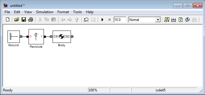
Pendulum diagram.

Let's add parameters to the Body block. The Body will be a 1 meter zero-thickness bar with a mass of 1 Kg. Double click the Body block and modify the parameters to match the following image.

Bar parameters.

Click apply and close this window. Now change the simulation time to 2 (seconds) and hit the play button. On the new window, click the "Enable automatic expanding fit" button to take a better view at the pendulum movement.

Simulating a pendulum.

Analyzing the pendulum


Now that we have a visual, I'll proceed to explain how the Coordinate Systems (CS) works.

The pendulum CSs.

Let's look at the big picture, we have the Ground, which is our reference point for this kinematic chain and is located at [0, 0, 0]. Next we have a Body (the bar) with two CSs (Coordinate Systems), each CS is attached to one particular point of the body as you can see.

The Ground and the Body are connected by a Revolute block, which is a joint. A joint is a relationship between two CS, one CS for each intervening body. The joint add restrictions between these two CS, because in 3D space an unrestricted CS has 6 DoF with respect to another CS. In our example the Revolute joint only allows 1 rotational DoF in the Z axis direction ([0, 0, 1]). This means that CS1 can't translate with respect to the Ground, i.e. it will remain at the global position [0, 0, 0], and can only rotate around the global Z axis.

Let's now analyze the Body parameters. We have three Coordinate Systems: CS1, CS2 and CG. The CG is the center of gravity and the other two CS are for reference/positioning. To specify the position of any CS we need:
  • A first CS, which I'll call the rCS: reference Coordinate System
  • A second CS, which I'll call the oCS: orientation Coordinate System
  • A [x, y, z] distance vector.
The position of the CS will be at a distance [x, y, z] starting from the rCS and moving along the XYZ axes of the oCS.

These 3 parameter allow great flexibility but also can add some confusion. To simplify your life and mine, we'll stick to the following convention:
  • We'll use the World CS as the oCS.
  • We'll use CS1 as the rCS for every CS, except for CS1. For CS1 we'll use Adjoining** as the rCS.
  • We'll also refrain from rotating bodies, i.e. we won't use the orientation tab of the body parameters.
** Adjoining can only be used at a CS that is part of a joint, and it does reference to the other CS that is part of the joint.

The final parameter is the moment of inertia, which is expressed as a tensor. The moment inertia must be taken at the CG and is expressed along the XYZ axes of the CG. For this example I assumed a zero thickness bar, you can find the most common moment of inertia at wikipedia.

The robotic arm


The previous section, understanding the position and orientation system, was the hardest of this tutorial. Now we can add the two missing members of our "robotic arm". In fact, I'm gonna let you do that as a homework, but I'll provide some hints.

XYZ Robot Diagram.

The "Robotic Arm" is composed of 3 zero-thickness bars, each one measure 1 m and weights 1 Kg. Each bar initial position is oriented along the X, Y an Z axes respectively. The joints of the robot are all Revolute and allow rotation in the Z, X and Y axes as the figure above shows.

Below there is an animation that shows the initial position of the robot.

XYZ Robot Initial Position

You can change the color of the bodies in the Visualization tab inside the Block Parameters of each body.

Collapse under gravity


After you've finished configuring your blocks, proceed to simulate the system. You'll see the robot collapses under gravity.

XYZ Robot collapsing under gravity.

To solve this problem, we'll use some basic control theory. The basic blocks of a control system are: sensors, actuators and controllers.

Adding sensors and actuators


Simmechanics provides an easy way to add sensors and actuators to the system. Start by double clicking any of the joint blocks of the robot.

Enabling sensor / actuator ports.

Enable 2 sensor / actuator ports on each joint. Next, hook a Joint Sensor and a Joint Actuator, you can find both blocks under the Sensors and Actuators category, to each joint. Finally, connect the output of each sensor to a Scope block, you can find it under Simulink > Sinks Category.

XYZ Robot with sensors.

Simulate the system, and take a look at each Scope, you'll see how much each body rotates with respect to its base (or predecessor body). Take a close look at the animation and the scopes and relate the sign of each signal with the rotational axis to which is associated.

Z Joint
X Joint
Y Joint

Closing the loop


We already plugged both the sensors and the actuators, the only part missing is the controller. We'll add to controller to maintain the initial position of the XYZ Robots, so it doesn't collapses under gravity.

We'll need the following blocks: The PID Controller block, found under the Simulink > Continuous; the Sum block, found under Simulink > Math operations; and the Constant block, found under Simulink > Sources. You'll need to modify the Sum block parameters, so the List of Signs is: "|+-".

Configuring the Sum block for subtraction.

Next, you'll need to wire the new blocks as shown in the next figure.

XYZ Robot with PID blocks.

The final step is tuning the gains of each PID block. After some trial and error, I ended with the following gains:

P
I
D
N
Z Joint
185
282
14
239
X Joint
121
197
6
435
Y Joint
17
27
1
423

All that's left is to check the correctness of the controller by simulating the system.

XYZ Robot fighting gravity with its PID controllers.

Z Joint
X Joint
Y Joint

What's next? (Homework for you)


I hope this simple and unrealistic example had accomplished its mission of teaching you the fundamentals of the Simmechanic toolbox.

If you want to keep playing, you can immediately do the following:
  • Change the reference signals X, Y and Z from a constant 0 to some time varying signal, like a step or a sine wave. You'll notice soon enough the controller will start misbehaving because of the high non-linearity of the system.
  • Remove the gravity and see how that affects the performance of the controller when tracking a time varying reference. You'll need to insert a Machine Environment block and enable the Machine Environment port of the Ground block.
With some hard work you can do the following:
  • Implement a better model for the actuators (motors), by adding limits to the torque and speed, and also adding moment of inertia and friction to the joints.
  • Build a more realistic robot/system. Here, CAD software like Solidworks help a lot, because you can extract real information like distances, masses and moments of inertia. For example you can find the CAD files of the robot I've shown at the beginning of this post here. You can add more realistic rendering to your model using .STL files.
  • Implement a more robust controller using techniques like computed torque or fuzzy logic.
  • Study about forward (see Denavit-Hartenberg) and inverse (see iterative methods) kinematics and implement some trajectory tracking routines for your robot.

Once you've done that, you'll be closer to simulating a humanoid robot.

Thursday, January 3, 2013

Beaglebone: Using an USB WiFi dongle to connect to wireless networks at boot.

I'll cover how I configured my BeagleBone so it now (automagically) connects to wireless networks at boot.

Note: I assume you are running Ubuntu 12.10 in your Beaglebone.

Manual connection


First, let's check whether the Beaglebone can use the WiFi dongle by setting up a manual connection.

Before starting the test, let's install some software with the ethernet cable plugged in:
#On the beaglebone
sudo apt-get install lshw
sudo apt-get install wpasupplicant
Now unplug the Ethernet cable from the Beaglebone. And start a connection using the USB emulated Serial connection.
# On the PC
screen /dev/<ttyUSBx> 115200
Now let's check if the Beaglebone has recognized the WiFi dongle.
# On the beaglebone
lshw -C network
I got this:
*-network:1 DISABLED
description: Wireless interface
physical id: 2
bus info: usb@1:1
logical name: wlan0
serial: d8:eb:97:12:e4:c0
capabilities: ethernet physical wireless
configuration: broadcast=yes driver=rtl8192cu driverversion=3.2.33-psp26 firmware=N/A multicast=yes wireless=IEEE 802.11bgn
If you see something similar, it means your device has been detected by the Linux kernel and an appropriate driver has been loaded.

Remember the logical name, in this case is wlan0.

Now, turn on the WiFi dongle. (Use the logical name obtained from the last command)
# On the beaglebone
sudo ifconfig wlan0 up

Blue LED indicates that the WiFi dongle has been turned ON.

Scan for visible WiFi networks.
# On the beaglebone
sudo iwlist wlan0 scanning
You should see your network in the list:
wlan0     Scan completed :
          Cell 01 - Address: 00:13:49:CA:F5:10
                    Channel:4
                    Frequency:2.427 GHz (Channel 4)
                    Quality=56/70  Signal level=-54 dBm
                    Encryption key:on
                    ESSID:"your-ssid"
                    ...
Now, let's connect to your network.
# On the beaglebone
sudo nano /etc/network/interfaces
Append or modify the file to include the following text (I'm assuming your network it's WEP protected):
auto wlan0
iface wlan0 inet dhcp
    wireless-essid <ssid>
    wireless-key s:<ascii key>
Next, start the connection
# On the beaglebone
sudo ifup wlan0
And finally, test the connection
# On the beaglebone
ping www.google.com

Congratulations, you have connected to a wireless network.

Going automatic


We'll use wpa_supplicant to automate the connections to wireless networks.

wpa_supplicant is a daemon that manages unsecure, WEP and WPA wireless connections.

wpa_supplicant stores the information about the wireless networks that it can connect to in a .conf file, usually named wpa_supplicant.conf.

You can create/edit it, using:
sudo nano /etc/wpa_supplicant/wpa_supplicant.conf
This is how it should look like:
ctrl_interface=/var/run/wpa_supplicant

# Unsecure Network
network={
    ssid="<ssid>"
    key_mgmt=NONE
    priority=<unsecure_priority>
}

# WEP Network
network={
    ssid="<ssid>"
    key_mgmt=NONE
    wep_key0="<key>"
    priority=<wep_priority>
}

# WPA Network
network={
    ssid="<ssid>"
    psk="<passphrase>"
    priority=<wpa_priority>
}

For more examples about the .conf file, check this website.

Let's reconfigure the network interface to add support for wpa_supplicant.
sudo nano /etc/network/interfaces
Change the wlan0 part to match the following text:
auto wlan0
iface wlan0 inet dhcp
    wpa-driver wext
    wpa-conf /etc/wpa_supplicant/wpa_supplicant.conf
Finally reboot the BeagleBone to see the changes.
sudo reboot
Done!

Monday, October 22, 2012

Beaglebone: Installing Ubuntu 12.10

I've got my hands on a Beaglebone, and the first thing I did was installing the latest Ubuntu 12.10 on it. Here how I proceeded.

This post is mainly for self-documenting, feel free to follow my footsteps at your own risk. These steps will probably also work on the Beagleboard.

Back up the original image


The Beaglebone comes with the Linux Ã…ngström distribution. So I backed up the original image, in case something failed. Even if I were to stick with the Ã…ngström distro, it's a good idea to back up the original image.

I removed the microSD that shipped with the Beaglebone, and inserted it into my PC SD slot. Then I checked in which partition it got mounted, using the following command.
df -l
/dev/sda is my PC harddrive, and /dev/sdb is the Beaglebone SD card.

After identifying where the SD was mounted, I used the following command to backup the SD.
dd if=/dev/<sdx> | gzip > /path/to/image.gz
In case I needed to restore the image, I'll have to use the following command:
gzip -dc /path/to/image.gz | dd of=/dev/<sdx>

Installing Ubuntu


I followed the instructions from elinux. These are the summarized steps:
  • Download the minimal Ubuntu 12.10 image
cd ~/Desktop
wget http://rcn-ee.net/deb/rootfs/quantal/ubuntu-12.10-r2-minimal-armhf-2012-11-29.tar.xz
  • Verify the integrity of the image
md5sum ubuntu-12.10-r2-minimal-armhf-2012-11-29.tar.xz
Which should match the following output
b0ee1964a3f8196f4f1a501d1d2ac83a ubuntu-12.10-r2-minimal-armhf-2012-11-29.tar.xz
  • Untar the package
tar xJf ubuntu-12.10-r2-minimal-armhf-2012-11-29.tar.xz
cd ubuntu-12.10-r2-minimal-armhf-2012-11-29
  • Flash the image into your SD
sudo ./setup_sdcard.sh --mmc /dev/<sdx> --uboot bone

Finished flashing the Ubuntu image into the SD card.

For the record (Older releases):

Release 1: http://rcn-ee.net/deb/rootfs/quantal/ubuntu-12.10-r1-minimal-armhf-2012-10-19.tar.xz
MD5: 31be6761a37af98906c5c1e892601e85

Connecting to your Beaglebone


After flashing the Ubuntu image, I removed the SD from my PC and plugged it back into the Beaglebone. I decided to make the first connection using the tty over USB.

After connecting the Beaglebone to my PC using a USB cable, I had to figure out the exact name of the ttyUSBx with the following command.
dmesg | grep ttyUSB
From documentation, ttyUSB0 -> JTAG, ttyUSB1 -> UART (terminal)

I used GNU screen to stablish the connection:
sudo apt-get install screen
screen /dev/<ttyUSBx> 115200
After the connection was established. I saw no output so I pressed the reset button on the Beaglebone.

Voilà

The default login information is below.
  • login: ubuntu
  • password: temppwd

Things to do after installing Ubuntu


OK, I logged in! ... Now what?

Change your password


First thing first, I changed the default password to something stronger
# On the Beaglebone
passwd

Connect the Beaglebone to the internet


I plugged an Ethernet cable into the Beaglebone, and checked if the connection was OK.
# On the Beaglebone
ping www.google.com
I let ping run for a while and then I finished it with Ctrl+C.
Notice the "0% packet lost", that's a Win.

OK I lied, it didn't work the first time, I got 100% packet lost, but resetting the Beaglebone solved the problem.

Autocompletion


Next, I enabled bash completion - a.k.a. the tab autocompletion:
# On the Beaglebone
sudo apt-get update && sudo apt-get install bash-completion

Change the hostname


The terminal prompt says "ubuntu@arm". This means the Beaglebone hostname is "arm". I changed that with the following commands.
# On the Beaglebone
cat /etc/hosts
I got the following output.
# On the Beaglebone
127.0.0.1 localhost
127.0.1.1 arm
So I changed the second line with:
# On the Beaglebone
sudo nano /etc/hosts
# changed the second line from arm to <new-hostname>
Next, I did:
# On the Beaglebone
cat /etc/hostname
And got:
# On the Beaglebone
arm
I changed that with:
# On the Beaglebone
sudo nano /etc/hostname
# changed the hostname from arm to <new-hostname>
Finally I rebooted the Beaglebone to apply the changes.
# On the Beaglebone
sudo reboot

Change your login name


Now the terminal prompt says "ubuntu@beaglebone", the login is "ubuntu". I also changed that.

I had to enable the root account:
# On the Beaglebone
sudo passwd root
# Entered a temporary password
Pressed "Ctrl + D" to logout and I logged as root:

Logging as root.

I changed the old username with:
# On the Beaglebone
usermod -l <new-username> ubuntu
I also added a comment to my new user:
# On the Beaglebone
usermod -c "<full-name-or-comment>" <new-username>
Next, I moved to my new home:
# On the Beaglebone
usermod -md /home/<new-username> <new-username>
Finally, I also renamed the "ubuntu" group to match my new username:
# On the Beaglebone
groupmod -n <new-username> ubuntu
I logged out (Ctrl + D) and logged with my new username:

Logged with my new username.

Finally I locked the root account:
# On the Beaglebone
sudo passwd -l root

Set up a zeroconf hostname


A zeroconf hostname, simplifies SSHing with a local machine by assigning it a hostname on the LAN. This way I don't need to know the IP (which can change over time) to start a SSH session.
#On the Beaglebone
sudo apt-get install avahi-daemon
Now I can connect to the BeagleBone via ssh using the following command:
# On the PC
ssh <beagle-username>@<beagle-hostname>.local

SSHing the Beaglebone


I finished the screen session, using Ctrl+A and then K. I rebooted the Beaglebone, this way the avahi daemon got launched on the next boot.

ssh jorge@beaglebone.local instead of ssh jorge@192.168.1.x

SSH login without password


Everytime I SSH'ed the Beaglebone I needed to input the Beaglebone login and password. The next commands got rid of that.
# On the PC
ssh-keygen # Don't enter a passphrase
ssh-copy-id <beagle-username>@<beagle-hostname>.local

SSH without login

Install GNU screen


I quickly found out that I needed multiple SSH sessions to open multiple terminals on the Beaglebone. Searching for a workaround I found GNU Screen.

With GNU screen I can create multiple "screens", with one terminal inside each of them. All this can be done with keyboard commands.
#On the Beaglebone
sudo apt-get install screen
To start screen I needed to use the following command on every login.
#On the Beaglebone
screen -S 1
This was annoying, so I automated the task:
# On the PC
gedit ~/.bashrc
I appended the following text:
Now with a single command, I can SSH login into the Beaglebone and enter in a running "screen" or create a new "screen", if it doesn't exists.
#On the PC
sshbeaglebone

SSH session with the Beaglebone splitted in 3 using screen.


Other important software


I also installed additional software:
#On the Beaglebone
sudo apt-get install man-db # Manuals
sudo apt-get install vim # Text editor
sudo apt-get install octave # Numerical package
sudo apt-get install build-essential # make, gcc, et al.

What's next?


Acknowledgements


Sunday, October 21, 2012

Ubuntu: How to add Eclipse to the Unity Launcher

A quick how to: Add Eclipse to the Unity Launcher. You can add any other application to the Unity Launcher using these steps.

All the Unity Launchers (e.g. evince, gedit, etc) are implemented as .desktop files. These files are stored in the folder /usr/share/applications/. The .desktop file contains the following information: where the icon is located, where the executable is located, the launcher name, and other secondary information like a comment about the launcher.

Make Eclipse accessible from the command line


All the commands accessible from the command line are stored in a "bin" folder. The folder destined to user binaries is located in /usr/bin.

Let's add the eclipse executable to /usr/bin using the following command.

sudo ln -s /path/to/eclipse/eclipse /usr/bin/

Now eclipse is accessible from the command line as the command eclipse.

Put the icon in the right place


All the icons associated to a Unity Launcher are stored in the /usr/share/pixmap folder. Let's place the eclipse icon in the right folder.

sudo cp /path/to/eclipse/icon.xpm /usr/share/pixmap/eclipse.xpm

Create the .desktop file


Finally, you'll need to create a new .desktop file for Eclipse. Proceed with the following command.

sudo gedit /usr/share/applications/eclipse.desktop

Insert the following text inside this new file.

Note 1: If you didn't add eclipse to /usr/bin, you'll have to use the full path in the Exec section, e.g. Exec=/path/to/eclipse/eclipse

Note 2: If you didn't place the eclipse icon under the /usr/share/pixmap folder, you'll have to use the full path in the Icon section, e.g. Icon=/path/to/eclipse/icon.xpm

This is the result.

Now, Eclipse is accessible from dash and the Unity Launcher.

Sunday, October 7, 2012

Windows: Installing qwt library

Qwt is a Qt based library that extends the Qt API with plotting capabilities.

Installation


 I'm assuming you have already installed MinGW (GCC compiler) and the Qt library, if you haven't then check this post.

Next you'll need to add the MinGW binaries to the PATH environment variable, if you haven't done so. If you don't know how to edit environment variables, check this post.

Append "C:\mingw\bin" (use the correct directory path) to the PATH variable.

Append "C:\Qt\4.8.3\bin" to the PATH variable.

Grab the latest qwt source (zip version) from here.

Unzip the zip file, go inside the qwt folder and open the qwtconfig.pri file with a text editor.

Comment (i.e. add a '#' character to the leftmost side) the following line:

QWT_CONFIG     += QwtDesigner

Save and close the .pri file.

Now open a command line window and type the following commands:

cd C:\path\to\downloaded\qwt
qmake
make
make install

Note: Instead of  "C:\path\to\downloaded\qwt" use the correct path like "C:\Users\Jorge\Downloads\qwt-6.0.1"

A new folder will be created in the C:\ drive named qwt-6.0.1 or similar.

The final step is updating the environment variables, if you don't know/remember how check this post.

Append "C:\qwt-6.0.1\include" to CPLUS_INCLUDE_PATH
Append "C:\qwt-6.0.1\lib" to LIBRARY_PATH

Note:  You won't be able to see the qwt widgets in Qt designer with these installation steps. I haven't figured out yet how to enable that.

How to use qwt

Create a new Qt project in Qt creator, and add to the .pro file the next line:

Linking qwt library

Next, you'll need the library header files, all of them start with "qwt_". Add them where necessary as shown in the next image:

Including qwt header files.

Simple test


Let's do a very simple test and see if everything has been installed correctly. In your mainwindow.cpp source file type the next code:

Simple test source code.

Then run it, and you should see the following output.

Simple test output.

Other Examples


For more elaborated examples check qSerialTerm and ImageQ.

 ImageQ in Windows. Histogram was plotted using QwtPlot.

Windows: Environment Variables for MinGW

Environment variables, as the name implies, are variables that hold directories paths as strings. Environment variables goal is to keep track of important files for the system.

In windows, the most important environment variable is the PATH variable. You can check its content on the command line using the following command:

echo %PATH%

Environment variables can also keep track of important files for the compiler (e.g. MinGW GCC) like header files and static and dynamic library files.

Adding, editing or deleting environment variables


To add, modify or delete an environment variable, you'll need to head to Control Panel > System > Advanced System Settings. On the Advanced tab, click on the Environment Variables... button.

The following window will pop out.

List of environment variables

Environment variables are divided in two groups: User variables and System variables. The most important group is the System group. You can create, modify or delete variables using the button New, Edit or Delete respectively.

Let's try editing the Path variable. Click on the Path variable in the System variables group and then click the Edit button.


As you can see, the variable is a list of directory paths separated by the ";" character. The most safe way of adding a new directory is by appending the path as follows:

;C:\mingw\bin

That way there won't be name crashes.

There are many environment variables, let's review the most important ones.

Binary path (PATH)


The PATH (or Path, Windows is case insensitive) variable holds paths to binary files like .exe files, to commands and to .dll files.

Be careful with this variable, do not delete the default path like System32 and so on. Generally, you'll only need to append new directory paths to this variable.

For example:

Append ";C:\mingw\bin" to the Path variable

Important note: Do NOT create a new Path or PATH (again, Windows is case insensitive) variable in the system variable group or you'll override the default paths and you'll be in trouble.

Include paths (CPLUS_INCLUDE_PATH, C_INCLUDE_PATH)


These variable hold the directory paths to header files (like library header files). Important for linking new installed libraries.

Generally you'll need to append the path to a library "include" folder.

For example:

Append ";C:\mingw\include" to the CPLUS_INCLUDE_PATH

CPLUS_INCLUDE_PATH and C_INCLUDE_PATH are pretty much the same. When the compiler looks for a header file, it looks in both variables. So having two variables is only useful for the programmer to keep things tidy.

Library path (LIBRARY_PATH)


This variable hold the directory paths to static library (.lib or .a files). This one is also important for linking new libraries.

Generally you'll need to append the path to a library "lib" folder.

For example:

Append ";C:\mingw\lib" to the LIBRARY_PATH

Saturday, October 6, 2012

How to: OpenCV in Qt creator and ImageQ

In this post I'll cover how to glue the OpenCV libraries to Qt creator via an example. And I'll also release ImageQ, a Qt based image processing application.

OpenCV


OpenCV is an open source library that contains various functions for computer vision and image processing. OpenCV is written in C/C++ but there are ports for Java and Python.

Qt framework


Qt is a framework for cross development of Graphical User Interfaces (GUI) in C++. Qt libraries are open source.

Qt creator is an Integrated Development Environment (IDE) for Qt applications. Qt creator was created using the Qt framework as well.

Dependencies


You'll need the following libraries/software:

  • Qt creator
  • Qt libraries
  • OpenCV libraries

Ubuntu


Open a linux terminal and type the following commands:

sudo apt-get install qtcreator # Qt creator + Qt libraries
sudo apt-get install libopencv-dev # OpenCV libraries

On Ubuntu 12.04 you'll end with Qt libraries version 4.8 and OpenCV libraries version 2.3.

Windows

First, you need Qt creator and Qt libraries. Follow the steps in this post and come back.

Now, grab and unzip OpenCV from here.

Next, install CMake (win32 exe) from here.

You'll need to add C:/mingw/bin to your PATH environment variable. Check this post for a how to.

Now, launch cmake-gui.

Select as source folder: The unzipped version of OpenCV and as build folder: any folder you want. Then click on the configure button, from the drop down menu select the MinGW makefiles and accept. You should get the following output.

OpenCV build configuration.

Go with the default configuration and click the generate button.

Now open a cmd and head to your "build folder" (the one you selected in CMake) and run the following command:

mingw32-make

Now go get a coffee, a sandwich or take a nap while the compiler does it job.

(coffee break)

OK, after thousands of compiler messages, you finally obtained the necessary binaries.

Execute the next command:

mingw32-make install

A new folder name "install" will be created in your "build folder". Copy the contents of this "install" folder in any folder you like (e.g. C:/opencv). You can now delete the "source code folder" (the one you download from OpenCV website) and the intermediate compiled objects (a.k.a. your "build folder").

Now you'll need to modify some environment variables. Check this post if you don't know how.

I'm assuming you are using the C:\opencv folder, change the path if necessary.

Append to the PATH (or Path, is the same, do NOT create a new variable) variable: C:\opencv\bin

Append to the CPLUS_INCLUDE_PATH variable: C:\opencv\include

Append to the LIBRARY_PATH variable: C:\opencv\lib

Setting up the Qt project


(The rest of the article is the same for Ubuntu and Windows users)
  • Launch Qt creator.
  • Start a new project (usually Qt Gui Application).
  • Head to your .pro file.
  • Inside the .pro file add these lines:

Linking OpenCV libraries (Linux)

Note: You probably won't need to link all the libraries, only link the ones you are going to use. The most common libraries are core, highgui and imgproc.

Adding the headers


OpenCV library headers are inside the opencv2 folder. To add these headers to your application add the following line:

Adding OpenCV library headers.

Displaying the images


OpenCV offers a function named cv::imshow for displaying images. However this method won't integrate to your Qt application.

In Qt, images are usually displayed in QLabels using the method setPixmap(). As the name implies the argument for this method must be a QPixmap object. QPixmap objects are optimized for displaying, meanwhile QImage objects are optimized for pixel manipulation. Using the static method QPixmap::fromImage() a QImage can be converted in a QPixmap.

Is easier to convert a cv::Mat, the basic OpenCV image object, to a QImage object than to a QPixmap objetc.

In summary, the necessary steps are listed below:

  • Convert the cv::Mat object to a QImage object.
  • Convert the QImage object to a QPixmap object, using QPixmap::fromImage().
  • Add the QPixmap object to a QLabel, using setPixmap().

To convert a cv::Mat to a QImage, you can use my implementation available on the following links: header and source.

An example


Let's put everything together in an example. Head to your .ui file and add a label (leave the default name "label"), as shown in the following image. (I have also added grid layout, not necessary but helps visualization)

Toy application layout

Next, add the mat2qimage.cpp and mat2qimage.h to your project.

Now, on your mainwindow.cpp source file type the following code:

Toy application source code.

Note: In Windows, I had to use the full path to the image and the '\' characters needed to be written as "\\" insted. Example: "C:\\Users\\Jorge\\Desktop\\myimage.JPG".

This is the output, after running the example:


Toy example output. (Image from wikipedia)

ImageQ


Using these basics, I have developed ImageQ in Qt. ImageQ provides GUI access to some basic OpenCV functions. You can use ImageQ to learn the basics of image processing or to experiment with OpenCV function parameters.

ImageQ: Coin image after Sobel operator.

You can get ImageQ source code from this github repository.

P.S. For ImageQ you'll also need Qwt libraries, you can install these in Ubuntu using the following command. (Windows users, check this post instead)

sudo apt-get install libqwt-dev